Assessing and Comparing Classifier Performance with ROC Curves in R for Data Science

This article shows how to use ROC curves and AUC in R to rigorously evaluate, compare, and threshold-tune classifiers so you can select models that align with real business trade-offs between false positives and false negatives.

Article Outline

1. Introduction Why evaluating classifiers goes beyond accuracy; how ROC curves illuminate the trade-off between sensitivity and specificity in real-world data science problems.

2. ROC Curve Fundamentals Definitions of True Positive Rate (TPR/Recall) and False Positive Rate (FPR); how thresholds generate the ROC curve; intuition for the diagonal baseline and the ideal top-left corner.

3. AUC (Area Under the ROC Curve) and Interpretation What AUC summarizes, how to read values from 0.5 (no skill) to 1.0 (perfect), ties to ranking quality, and when AUC is preferable to accuracy or F1.

4. R Environment Setup Required packages and roles: tidyverse for data handling/plots, pROC (and/or yardstick) for ROC/AUC, caret for consistent modeling APIs, plus model packages (e.g., glm/stats for logistic regression, ranger for random forest, e1071 for SVM).

5. Data Preparation Constructing a binary classification dataset with informative and noisy predictors; train/test split; class balance checks; creating a tidy evaluation frame for later plotting.

6. Training Multiple Classifiers in R Fitting logistic regression (glm), random forest (ranger via caret), and SVM (e1071 via caret); extracting calibrated probabilities or decision scores for ROC analysis.

7. Building ROC Curves in R Computing ROC points and AUC with pROC::roc; plotting multiple ROC curves on one figure; adding confidence intervals and a reference diagonal; tidy approach with yardstick.

8. Comparing Models with AUC and Statistical Tests Interpreting overlapping curves; partial AUCs (high-specificity regions); DeLong test to compare AUCs; business-context discussion of false positives vs. false negatives.

9. Choosing Operating Thresholds Finding thresholds with Youden’s J statistic; optimizing for cost-sensitive objectives; translating thresholds to expected confusion matrices on the test set.

10. End-to-End Example in R Complete script: dataset generation → model training → probability predictions → ROC/AUC computation → multi-model ROC plot → threshold selection and confusion matrices.

11. Common Pitfalls & Best Practices ROC on imbalanced data (contrast with Precision-Recall curves); leakage and nested resampling; averaging across folds; setting seeds for reproducibility; plotting clarity.

12. Conclusion & Next Steps Recap of ROC/AUC for model selection; guidance on extending to cross-validation summaries, PR curves, calibration curves, and cost-based model selection frameworks.

Introduction

In data science, selecting the right classification model often involves a trade-off between multiple performance metrics. Accuracy alone does not always capture the nuances of model quality, especially in imbalanced datasets. Receiver Operating Characteristic (ROC) curves offer a visual and quantitative method to evaluate and compare classifiers across different thresholds, highlighting sensitivity-specificity trade-offs. This article provides a comprehensive exploration of ROC curves, the Area Under the Curve (AUC), and their use in comparing classifiers in R, complete with an end-to-end example using a simulated dataset.

ROC Curve Fundamentals

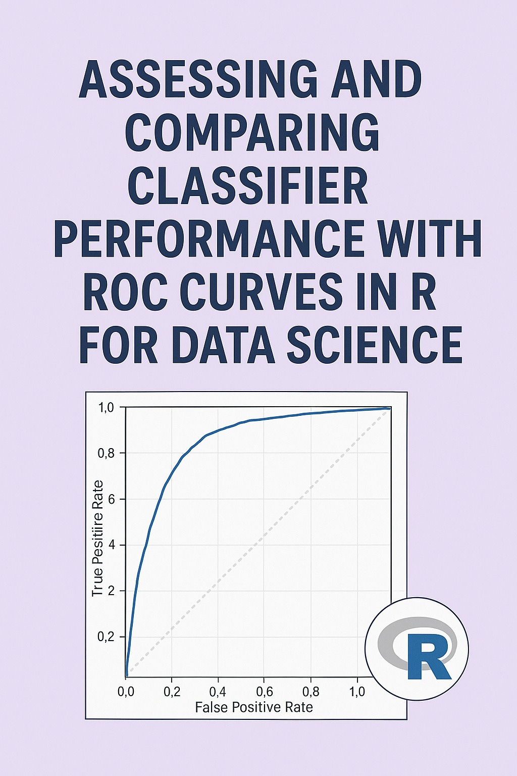
The ROC curve plots the True Positive Rate (TPR, or sensitivity) against the False Positive Rate (FPR, or 1-specificity) at different classification thresholds. TPR measures the proportion of actual positives correctly identified, while FPR measures the proportion of actual negatives incorrectly classified as positive. By varying the threshold, we trace out the ROC curve, from the lower left corner (all negative predictions) to the upper right corner (all positive predictions). A model with perfect classification ability would reach the top-left corner.

---

---